WaBis
walter.bislins.ch
Determining the Shape of the Earth with Zenith Angle Measurements

Problem
If we assume that light travels in straight lines we could easily recognize the real shape of the earth and calculate its size by using a theodolite to measure the drop of a target or the horizon. On a Flat Earth the drop is zero on the Globe it is about d2 / 2R, where d = distance to target and R = radius of the earth.
But we have an atmosphere which refracts light up or down. What a theodolite sees is not the real geometry of the earth, but an up or down refracted image. Whatever the shape of the earth is, we will always see a distorted image of the earth due to refraction. So how can we measure how much curvature is due to the shape of the earth and how much is due to refraction?
If we can measure refraction somehow, we can correct the apparent curvature and get the real geometry of the earth.
Note: there are devices that can measure refraction directly, e.g. by using 2 lasers of different wavelengths. So we know the earth is a Globe not at last from such measurements. [1]
Method
Refraction depends on the atmospheric condition between observer and target. We can approximate the light rays between observer and target through an arc with a radius of curvature r.
We can use the method of simultaneous reciprocal zenith angle measurements using 2 theodolites to measure the apparent drop the theodolites see each other. The drop is measured as the angle from the vertical to the target. The angle is called the Zenith Angle. The sum of the measured zenith angles depends on the shape of the earth and the radius of curvature of the light ray. So if we know the shape and size of the earth, we can calculate the refraction from the zenith angle measurements.
Now we pretend not to know the shape of the earth. But we can calculate the curvature of the light ray for both models anyway and then use a physical model of the atmosphere to calculate the atmospheric parameters that result in this curvature. Then we can measure the real parameters like the temperature, pressure and temperature gradient and show for which earth model the real values can match the calculations.
If the real conditions can't produce the curvature of the light that is calculated for one or the other earth model, than that model is false.
So lets see how this works.
Calculating the Curvature of a Light Ray
The curvature of light due to atmospheric refraction is very small. The radius of curvature is typically about 40,000 km. Because we often want the radius of curvature of light compared to the radius of the earth, it is practical to introduce a so called refraction coefficient k:
| (1) |
|
per definition | ||||||||||||
| where' |
| |||||||||||||
Although a Flat Earth has no curvature, the refraction coefficient can still be used in refraction calculations. We can always get the curvature of light from k as follows: r = 6371 km / k.
Because refraction itself does not depend on the shape of the earth, we can derive all calculations without assuming the shape of the earth.
We first need the connetion between the curvature of a light ray and the corresponding refraction angle. Then we can derive equations for the refraction angle from the zenith angles for Globe and Flat Earth model. Lets start:
Light Ray Curvature and Refraction Angle
The light ray curvature is not dependent on the earth model and can be calculated from the refraction angle as follows.

The magenta line is the direct line of sight from the observer to a target. The orange arc is the corresponding refracted light ray with radius of curvature r. The refraction angle is ρ (greek r, spelled rho) and the distance to the target is d.
Although the sketch shows a Globe model, the light ray geometry has nothing to do with the shape of the earth. The radius of the earth R does not appear in the equations below.
We have a right angle triangle r, d/2, b with an angle ρ. We can use trigonometry to calculate the sine of ρ:
| (2) |
The curvature c of the bent light rays is very small so the radius of curvature r = 1 / c is very big. We have very small refraction angles ρ if d is much smaller than r, which is the case in survey. For small angles ρ we can approximate sin(ρ) ≈ ρ:
| (3) |
The curvature of the light ray is the inverse of the radius of curvature. So we can solve (3) for 1/r:
| (4) |
| ||||||||||||
| where' |
|
Refraction Angle for the Globe Model
Now we derive the equation for the refraction angle

Assuming we have measured both zenith angles in degrees and assuming the radius of the earth is R we can get the refraction angle
| (5) |
Rearranging for
| (6) |
The angle
| (7) | ||||||||||
| where' |
|
Inserting this into (6) and solving for the refraction angle
| (8) |
| ||||||||||||
| where' |
|
We can now insert the refraction angle into the equation (4) for the curvature of a light ray:
| (9) |
This can be simplified to:
| (10) |
| |||||||||||||||
| where' |
|
This is the equation to calculate the curvature of a light ray from the simultaneously measured zenith angles for the Globe model.
We can get the commonly used refraction coefficient k as follows:
| (11) |
|
Note: if the light ray is straight, the right term above is equal −1 so the refraction coefficient for unrefracted light is k = 0.
Refraction Angle for the Flat Earth Model
We can use equation (11) for the Flat Earth model with a little correction. Because the verticals at the 2 locations on the Flat Earth are parallel, the tilt angle
| (12) |
| ||||||
| where' |
|
Similar as above we can now calculate the equation for the curvature of a light ray from the simultaneously measured zenith angles for the Flat Earth model:
| (13) |
| ||||||||||||
| where' |
|
This is alomost the same equation as for the Globe model (10), but the 1 / R term does not appear.
We can even calculate a refraction coefficient for the Flat Earth with the same definition
| (14) |
|
which is the same as the refraction coefficient for the Globe model (11) minus 1. So whenever we have a refraction coefficient for the Globe, e.g. in the Advanced Earth Curvature Calculator, we can calculate the corresponding Flat Earth refraction coefficient as:
| (15) |
|
Note: in reality the sum of the zenith angles is almost always measured greater than 180°. This means the curvature of the light ray on the Flat Earth model is negative, so the atmospheric conditions have to be such, that light gets bent upwards. This means that the air density has to increase with increasing altitude, which is not the case in reality.
But lets investigate the atmospheric conditions neccessary for a given zenith angle observation for the Globe and the Flat Earth:
Calculating the Temperature Gradient
The curvature of the light in the atmosphere is due to a gradient in the refractive index. The refractive index depends on air density, which is dependent via the ideal gas law on pressure and temperature, on the wavelenght of light and to a very small extent on humidity and CO2 concentration.
Because refraction does fluctuate in practice all the time, for practical calculations humidity and CO2 concentration can be ignored and the wavelength of green light is used. Try my Calculator for Refractivity based on Ciddor Equation and play with the sliders to see how much the influence of each parameter on the refractive index is.
Knowing the connection between atmospheric conditions and the refractive index (Ciddor Equation), using calculus we can derive the curvature of a light ray passing through an atmosphere with a certain density gradient, see Deriving Equations for Atmospheric Refraction.
The following equation gives the local curvature of a light ray depending on the atmospheric conditions at the location. If the conditions are about the same from the observer to the target, we can use this curvature for the whole path. In geodesy the inclination angle of a light ray is always near zero, so the influence of this angle (factor cos(≈0°) = 1) can be ignored.
| (16) |
| |||||||||||||||
| where' |
|
Note that this equation does not depend on the shape of the earth. Refraction is independent of the shape of the earth. So we can use this equation for the Globe and Flat Earth model.
I have shown how we can calculate the curvature of light from measurements of the zenith angles for the Globe and Flat Earth model.
If we solve the equation (16) above for the temperature gradient, we can then insert the calculated light ray curvatures to calculate the temperature gradient neccessary to bend the light ray accordingly:
| (17) |
| ||||||||||||
| where' |
|
This equation is independent of the shape of the earth as well.
Real Observations
To calculate the Globe an Flat Earth results the Calculator below was used. The elevation (Elev) is the mean elevation of the 2 stations. It's not the observer height above the ground. The Barometric Calculator was used to calculate pressure and temperature for this mean elevation. The Baromentric Calculator assumes the International Standard Atmosphere.

Note: The observer height is very important to get out of the strong refraction layer, see Refraction Coefficient as a Function of Altitude. For observations over great distances not over a flat landscape or water the line of sight is commonly for the most part way above the ground layer, so we can expect standard refraction, as the values in the table below confirm. On short distance measurements with observer heights around 2 m, the light rays travel in most cases the whole distance in the ground layer, where refraction can be considerably different than standard in both direction, which is confirmed by the Problematic Observations.
| Measurements | Globe Model | Flat Earth Model | ||||||||||
|---|---|---|---|---|---|---|---|---|---|---|---|---|
| Src | ζ1 | ζ2 | Dist [km] | Elev [m] | ρ | r [km] | k | dT/dh [°C/km] | ρ | r [km] | k | dT/dh [°C/km] |
| NGS | 91°08'09" | 89°07'44" | 32.139 | 2273 | 43.8" | 75,745 | 0.084 | −18.0 | -7'56.5" | −6956 | −0.916 | −211 |
| NGS | 91°03'44" | 89°15'34" | 39.476 | 2188 | 1'00.0" | 67,821 | 0.094 | −16.3 | -9'39.0" | −7032 | −0.906 | −208 |
| NGS | 90°40'36" | 89°56'32" | 76.957 | 2308 | 2'11.8" | 60,235 | 0.106 | −13.8 | -18'34.0" | −7125 | −0.894 | −208 |
| NGS | 90°32'21" | 90°12'12" | 92.882 | 2421 | 2'47.1" | 57,342 | 0.111 | −12.6 | -22'16.5" | −7167 | −0.889 | −208 |
| NGS | 90°49'49" | 89°45'41" | 74.362 | 2209 | 2'18.8" | 55,270 | 0.115 | −12.1 | -17'45.0" | −7201 | −0.885 | −205 |
| NGS | 90°50'01" | 89°35'13" | 52.518 | 2269 | 1'33.2" | 58,146 | 0.110 | −13.1 | -12'37.0" | −7155 | −0.890 | −206 |
| NGS | 91°09'00" | 89°22'35" | 66.128 | 2043 | 2'03.0" | 55,462 | 0.115 | −12.5 | -15'47.5" | −7198 | −0.885 | −202 |
| JK1 | 90°00'33" | 90°00'34" | 2.228 | 0.84 | 2.6" | 89,324 | 0.071 | −22.6 | -33.5" | −6860 | −0.929 | −186 |
| JK1 | 90°00'29" | 90°00'27" | 2.228 | 0.84 | 8.1" | 28,468 | 0.224 | 2.16 | -28.0" | −8208 | −0.776 | −161 |
| LS | 88°57'58.2" | 91°09'55" | 17.824 | 387 | 51.9" | 35,397 | 0.180 | −4.13 | -3'56.6" | −7769 | −0.820 | −172 |
This observations were done over great distances with a line of sight over 30 m above the ground, so the temperature gradient dT/dh was not influenced by ground effects.
Observations from the Transcontinental Triangulation of the American Arc of Parallel
The following table shows an extract from a much bigger table with more details of the page Refraction at the Transcontinental Triangulation of the American Arc of Parallel. The data is collected from measurements done at the Transcontinental Triangulation and the American Arc of the Parallel (PDF), published in 1900.
| Measurements Transcontinental Triangulation American Arc of Parallel | Calculations Globe | Calculations Flat Earth | |||||||
| Stations From-To | Dist [km] | ζ1 [deg] | ζ2 [deg] | Elevmean [m] | Rapparent [km] | k | dT/dh [°C/km] | k | dT/dh [°C/km] |
|---|---|---|---|---|---|---|---|---|---|
| Adobe-Cramers Gulch | 34.163 | 90.089167 | 90.187556 | 1549.0 | 7072 | 0.098 | -12.8 | -0.902 | -231.5 |
| Adobe-Square Bluffs | 30.701 | 89.877139 | 90.384667 | 1581.6 | 6717 | 0.050 | -23.9 | -0.949 | -230.4 |
| Adobe-Aroya | 35.218 | 90.269472 | 90.015028 | 1401.5 | 7091 | 0.101 | -14.9 | -0.899 | -207.6 |
| Antelope-Pilot Peak | 156.762 | 90.144972 | 91.082194 | 2496.5 | 7316 | 0.128 | -6.5 | -0.871 | -223.6 |
| Antelope-Deseret | 65.696 | 89.075806 | 91.440417 | 2556.2 | 7288 | 0.125 | -7.1 | -0.875 | -225.0 |
| Antelope-Ogden Peak | 38.546 | 88.799778 | 91.501500 | 1915.3 | 7328 | 0.130 | -6.8 | -0.870 | -218.9 |
| Antelope-City Creek | 33.063 | 90.358333 | 89.895806 | 2003.1 | 7451 | 0.144 | -4.8 | -0.856 | -209.6 |
| Antelope-Promontory | 41.044 | 90.159778 | 90.158889 | 1915.3 | 7377 | 0.135 | -5.6 | -0.864 | -217.8 |
| Antelope-Waddoup | 28.391 | 91.535528 | 88.680611 | 1901.9 | 7523 | 0.152 | -2.0 | -0.847 | -213.9 |
| Antelope-Salt Lake SE Base | 18.647 | 92.303278 | 87.842722 | 1585.5 | 7316 | 0.128 | -6.9 | -0.872 | -220.6 |
| Antelope-Salt Lake NW Base | 18.670 | 92.284528 | 87.862861 | 1572.6 | 7256 | 0.121 | -8.1 | -0.879 | -224.5 |
| Aroya-Hugo | 41.775 | 89.994528 | 90.343944 | 1504.6 | 7070 | 0.098 | -15.2 | -0.902 | -210.3 |
| Aroya-Eureka | 33.840 | 90.226944 | 90.046167 | 1338.2 | 7098 | 0.101 | -14.9 | -0.898 | -206.1 |
| Big Springs-Pikes Peak | 69.422 | 88.299111 | 92.249556 | 3063.7 | 7246 | 0.120 | -5.7 | -0.880 | -244.5 |
| Big Springs-Divide | 41.982 | 89.684361 | 90.654028 | 2179.3 | 7106 | 0.102 | -11.2 | -0.897 | -236.7 |
| Big Springs-Plateau | 47.805 | 90.502000 | 89.883000 | 1923.6 | 7112 | 0.103 | -11.4 | -0.897 | -233.3 |
| Big Springs-Holcolm Hills | 28.354 | 89.639056 | 90.595028 | 2077.1 | 6938 | 0.081 | -17.0 | -0.919 | -231.9 |
| Bison-Pikes Peak | 59.102 | 89.742667 | 90.734722 | 3765.5 | 7089 | 0.100 | -9.3 | -0.899 | -258.8 |
| Bison-Divide | 87.142 | 91.355333 | 89.342222 | 2887.6 | 7154 | 0.108 | -8.6 | -0.891 | -245.0 |
| Bison-Mount Elbert | 82.966 | 89.912806 | 90.755694 | 3815.1 | 7106 | 0.102 | -8.5 | -0.897 | -259.8 |
| Bison-Mount Ouray | 110.377 | 90.201250 | 90.689778 | 3756.7 | 7093 | 0.101 | -8.9 | -0.899 | -261.2 |
| Carson Sink-Mount Como | 123.697 | 90.461667 | 90.525028 | 2585.1 | 7180 | 0.112 | -8.8 | -0.888 | -237.5 |
| Carson Sink-Pah Rah | 108.825 | 90.519806 | 90.331972 | 2485.8 | 7317 | 0.128 | -6.1 | -0.871 | -226.0 |
| Carson Sink-Mount Grant | 122.287 | 90.140250 | 90.827722 | 2903.3 | 7235 | 0.118 | -7.2 | -0.881 | -236.3 |
| Carson Sink-Toiyabe Dome | 112.907 | 89.990417 | 90.914944 | 3028.0 | 7142 | 0.107 | -9.1 | -0.893 | -245.0 |
Conclusion
For the Flat Earth model we get required temperature gradients dT/dh of around −200°C/km and more. Such steep gradients are only possible in a ground layer with a hot surface and cool air above. The consistantly measured spherical shape of the earth (apparent radius about 7200 km) demands such a gradient in every altitude on the Flat Earth. This is physically impossible because the temperature would reach absolute zero below 2 km altitude.
On the Globe model however the calculated temperature gradients match the predictions of the accepted model for atmospheric refraction. According to a realistic atmospheric model the gradients will fade to about −6.5°C/km to −13°C/km of the standard atmosphere in the lower 30 m above the ground and maintain this gradient up to about 11 km, see Refraction Coefficient as a Function of Altitude. Due to decreasing air density with increasing altitude, refraction decreases with altitude even with a constant temperature gradient. The range of refraction of k = 0.07..0.2 with a mean value of 0.13 corresponds to standard refraction.
If we measure at least 30 m above ground level, we get consistent refraction with not much variation, see Refraction Coefficient as a Function of Altitude. This is well documented in the Observations from the Transcontinental Triangulation of the American Arc of Parallel, where all measurements werde done on towers, mountains or hills, way above the surface.
This measurements show that the earth cannot be flat. The required temperature gradients to produce real observations are physically impossible on a Flat Earth. The calculated temperature gradients for the Globe on the other hand are in the neighborhood of the expected gradient −6.5°C/km to −13°C/km of the standard atmosphere.
Problematic Observations
If the observer measures over relatively short distances from a height of about 2 m, the light travels in the ground layer of the atmosphere, where the ground exchanges heat with the air above, creating steep temperature gradients and hence strong refraction.
If the ground is cooler than the air, e.g. in the evening when the ground cools down faster than the air above, the gradient is always strong enough to bend light along the surface for hundreds of km. So it is no surprise, that on the Globe earth we can see lasers from behind the curvature in any distance. The nearer to the ground the observer and laser are, the stronger refraction is.
This ground effect is very well supported by the measurements in the following table, where all observations were done over short distances (dist) from below 30 m observer height (ht). This measurements are inconclusive to tell the shape of the earth, although the Flat Earth temperature gradients are much more pronounced.
| Measurements | Globe Model | Flat Earth Model | |||||||||
|---|---|---|---|---|---|---|---|---|---|---|---|
| Src | ζ1 | ζ2 | H [m] | Dist [m] | Elev [m] | ρ | k | dT/dh [°C/km] | ρ | k | dT/dh [°C/km] |
| JK2b | 90°00'11" | 90°01'00" | 1.7 | 1538 | 16.5 | -10.60" | −0.426 | −104 | -35.50" | −1.426 | −267 |
| JK2c | 89°40'31" | 90°19'58" | 1.6 | 1100 | 114 | 3.31" | 0.186 | −3.8 | -14.50" | −0.814 | −168 |
| JK2c | 90°22'18" | 89°37'51" | 1.6 | 150 | 110 | -2.07" | −0.853 | −174 | -4.50" | −1.853 | −339 |
| JK2c | 89°43'56" | 90°16'18" | 1.6 | 275 | 110 | -2.55" | −0.572 | −128 | -7.00" | −1.572 | −293 |
| JK2d | 90°14'24" | 89°45'43" | 1.6 | 143 | 11.8 | -1.19" | −0.512 | −118 | -3.50" | −1.512 | −281 |
| JK2d | 89°55'25" | 90°04'41" | 1.6 | 129 | 12 | -0.91" | −0.437 | −105 | -3.00" | −1.437 | −269 |
| JK2e | 90°04'32" | 89°55'33" | 1.6 | 61 | 5.6 | -1.51" | −1.536 | −285 | -2.50" | −2.536 | −448 |
| JK2e | 87°57'53" | 92°02'12" | 1.6 | 61 | 6.7 | -1.52" | −1.538 | −285 | -2.50" | −2.538 | −448 |
| JK2f | 90°21'16" | 89°38'48" | 1.6 | 150 | 28.4 | 0.43" | 0.176 | −5.33 | -2.00" | −0.824 | −169 |
| JK2f | 90°35'41" | 89°25'27" | 1.8 | 1000 | 23.7 | -17.81" | −1.10 | −234 | -34.00" | −2.10 | −377 |
| JK2f | 90°59'21" | 89°00'47" | 1.6 | 250 | 25.7 | 0.05" | 0.012 | −32.3 | -4.00" | −0.988 | −196 |
| JK2f | 90°33'15" | 89°27'04" | 1.6 | 500 | 21.1 | -1.40" | −0.173 | −62.6 | -9.50" | −1.17 | −226 |
| JK2f | 90°27'37" | 89°32'47" | 1.7 | 600 | 21.1 | -2.29" | −0.235 | −72.7 | -12.00" | −1.24 | −236 |
| JK2f | 89°59'04" | 90°01'03" | 1.6 | 100 | 18.8 | -1.88" | −1.16 | −224 | -3.50" | −2.16 | −387 |
| JK2i | 90°00'22" | 90°00'04" | 1.6 | 1538 | 16.5 | 11.9" | 0.478 | 43.7 | -13.0" | −0.522 | −119 |
| JK2i | 90°00'09" | 89°59'54" | 1.6 | 1538 | 16.5 | 23.4" | 0.940 | 119 | -1.5" | −0.060 | −441 |
Note: Because the refraction error increases with the square of the distance, for short enough distances the error l is small enough to be not a problem.
| (18) |
| ||||||||||||
| see |
Refraction Angle and Lift ( | ||||||||||||
| where' |
|
 Rainy Lake Experiment: Equations)
We can calculate the maximal distance to assure a certain accuracy even with high refraction. Measuring multiple times at different times a day and average over the measurements can give very good results. To do so we solve (18) for d and set l to the maximal error we accept.
Calculator
The calculator is preset for the first observation JK1 above. You can inspect the Calculator Code below.
Data Sources
National Geodetic Survey
| ID | Date | Project | Description |
|---|---|---|---|
| a | 1977 | NGS - McDonald Observatory | Long distance (32..93 km) observations at about 2000 m elevation, line of sight above 30 m |
 NGS Zenith Angle Measurements from the McDonald Observatory (PDF)
Survey of the McDonald Observatory Radial Line Scheme by Relative Lateration Techniques
NOAA Technical Report (PDF), June 1978
The NOS/NGS performed a special survey in the vicinity of the University of Texas McDonald Observatory. This was the initial phase of an extensive geodetic-geophysical study to detect any motions of the observatory relative to prominent topographic features within a region extending as far as 100 km from the observatory.
Very Long Line EDM & Reciprocal Zenith Angle Observations A Measure Of The Plumbline Tilt
Because that report included their reciprocal zenith angles (they call them zenith distances), I chose to include that set (see JK2a) and I personally knew Charlie Glover who performed that work. Here is a blog entry I made to share that information. ~ Jesse Kozlowski
Jesse Kozlowski Dataset JK1

 Observation Data Jesse Kozlowski
Flat Earth Proof? Perfectly Flat Level Lake by Jesse Kozlowski
Detailed documentation of the measurements and all data of the observation
Jesse Kozlowski Dataset JK2
| ID | Date | Project | Description |
|---|---|---|---|
| a | 1977 | NGS - McDonald Observatory | Long distance (32..93 km) observations at about 2000 m elevation, line of sight above 30 m |
| b | NOV 09 2015 | RTE 206 MP 27 & 28 | d = 1500 m, observer height 1.6 m |
| c | MARCH 08 2016 | Clarksville EDM CBL | d = 275..1000 m, observer height 1.6 m |
| d | MARCH 30 2016 | HAINESPORT "L" SHAPE | d = 130..142 m, observer height 1.6 m |
| e | APRIL 20 2016 | 200 FOOT "L" SHAPE | d = 60 m, observer height 1.6 m |
| f | OCT 07 2016 | Folsom EDM CBL S8 | d = 100..1000 m, observer height 1.6 m |
| g | OCT 20 2016 | Union Lake GNSS T2 | d = 760 m, observer height 1.4 m |
| h | NOV 01 2016 | Cooper River Lake | d = 2200 m, observer height 1.6 m |
| i | NOV 6-17 2016 | RTE 206 MP 27&28 LEVEL LINE | d = 1500 m, observer height 1.6 m |
Larry Scott
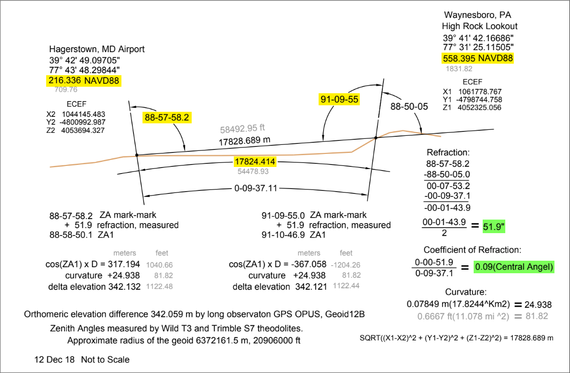 Reciprocal Zenith Angle Measurements from Waynesboro, PA High Rock Lookout to Hagerstown, MD Airport
Calculator Code
var Model = {
R: 6371000,
z1: 90.00916667,
z2: 90.00944444,
d: 2228.4,
P: 1013.25, // mbar
T: 15, // °C
rho_gl: 0,
rho_fe: 0,
r_gl: 0,
r_fe: 0,
c_gl: 0,
c_fe: 0,
k_gl: 0,
k_fe: 0,
dTdh_gl: 0,
dTdh_fe: 0,
Update: function() {
// Globe model
var TK = this.T + 273.15;
var a = (180 - (this.z1 + this.z2)) * Math.PI / 180;
this.rho_gl = this.d / 2 / this.R + 0.5 * a;
this.c_gl = 2 * this.rho_gl / this.d;
this.r_gl = 1 / this.c_gl;
this.k_gl = this.c_gl * this.R;
this.dTdh_gl = 12660 * this.c_gl * TK*TK / this.P - 0.0343;
// Flat Earth model
this.rho_fe = 0.5 * a;
this.c_fe = a / this.d;
this.r_fe = 1 / this.c_fe;
this.k_fe = this.c_fe * this.R;
this.dTdh_fe = 12660 * this.c_fe * TK*TK / this.P - 0.0343;
ControlPanels.Update();
},
};
ControlPanels.NewPanel( {
Name: 'InputPanel',
ModelRef: 'Model',
NCols: 2,
OnModelChange: function(field) { Model.Update(field) },
Format: 'std',
Digits: 5,
ReadOnly: false,
PanelFormat: 'InputNormalWidth'
} ).AddHeader( {
Text: 'Enter Zenith Angles, Distance, Pressure and Temperature',
ColSpan: 4,
} ).AddTextField( {
Name: 'z1',
Label: 'ζ<sub>1</sub>',
Format: 'dms',
ConvToModelFunc: function(s){ return NumFormatter.DmsStrToNum(s); },
Digits: 5,
} ).AddTextField( {
Name: 'z2',
Label: 'ζ<sub>2</sub>',
Format: 'dms',
ConvToModelFunc: function(s){ return NumFormatter.DmsStrToNum(s); },
Digits: 5,
} ).AddTextField( {
Name: 'd',
Label: 'Distance',
Units: 'm',
} ).AddTextField( {
Name: 'R',
Label: 'Radius Earth',
Units: 'km',
Mult: 1000,
} ).AddTextField( {
Name: 'P',
Label: 'Pressure',
Units: 'mbar',
Digits: 6,
} ).AddTextField( {
Name: 'T',
Label: 'Temperature',
Units: '°C',
} ).Render();
ControlPanels.NewPanel( {
Name: 'OutputPanel',
ModelRef: 'Model',
NCols: 2,
OnModelChange: function(field) { Model.Update(field) },
Format: 'std',
Digits: 5,
ReadOnly: true,
PanelFormat: 'InputNormalWidth'
} ).AddHeader( {
Text: 'Results',
} ).AddHeader( {
Text: 'Globe',
} ).AddHeader( {
Text: '',
} ).AddHeader( {
Text: 'Flat Earth',
} ).AddTextField( {
Name: 'rho_gl',
Label: 'Refr.Angle ρ',
Mult: Math.PI / 180,
Format: 'dms',
Digits: 6,
} ).AddTextField( {
Name: 'rho_fe',
Label: 'ρ',
Mult: Math.PI / 180,
Format: 'dms',
Digits: 6,
} ).AddTextField( {
Name: 'c_gl',
Label: 'Light Curve c=1/r',
Format: 'sci',
Units: '/m',
} ).AddTextField( {
Name: 'c_fe',
Label: 'c',
Format: 'sci',
Units: '/m',
} ).AddTextField( {
Name: 'r_gl',
Label: 'Light Curve r',
Units: 'km',
Mult: 1000,
} ).AddTextField( {
Name: 'r_fe',
Label: 'r',
Units: 'km',
Mult: 1000,
} ).AddTextField( {
Name: 'k_gl',
Label: 'Refr.Coeff k',
} ).AddTextField( {
Name: 'k_fe',
Label: 'k',
} ).AddTextField( {
Name: 'dTdh_gl',
Label: 'Temp.Gradient dT/dh',
Units: '°C/km',
Mult: 0.001,
} ).AddTextField( {
Name: 'dTdh_fe',
Label: 'dT/dh',
Units: '°C/km',
Mult: 0.001,
} ).Render();
xOnLoad( function() { Model.Update(); } );
Python Code
# dervation of equations:
#  http:#walter.bislins.ch/bloge/index.asp?page=Determining+the+Shape+of+the+Earth+with+Zenith+Angle+Measurements

import math

# input
# h1, h2 = altitudes of 2 observers in m
# z1, z2 = zenith angles of 2 observers in degrees
# d = distance between 2 observers in m

# output
# rho = refraction angle in rad
# c = curvature of light rays = 1 / radius of curvature
# k = refraction coefficient
# dTdh = temperature gradient in °C/m
# ?_gl for Globe
# ?_fe for Flat Earth

# constant
R = 6371000

# barometric equations for h = 0..11000 according to International Standard Atmosphere
# if don't have the altitudes use
#  T = 288.15
#  P = 1013.25
h = (h1 + h2) / 2
T = 288.15 - 0.0065 * h
P = 1013.25 * math.pow( ( 288.15 - 0.0065 * h ) / 288.15, 5.26 )

# common
a = (180 - (z1 + z2)) * math.pi / 180

# Globe model
rho_gl  = d / 2 / R + 0.5 * a
c_gl    = 2 * rho_gl / d
k_gl    = c_gl * R
dTdh_gl = 12660 * c_gl * T*T / P - 0.0343

# Flat Earth model
rho_fe  = 0.5 * a
c_fe    = a / d
k_fe    = c_fe * R
dTdh_fe = 12660 * c_fe * T*T / P - 0.0343
References
https://www.semanticscholar.org/paper/REFRACTION-INFLUENCE-ANALYSIS-AND-INVESTIGATIONS-ON-Boeckem-Flach/a53c08e2d9c2f2c8a4feb87002f6bc4646fe04e0